Forecasting & Optimization: A Mathematical Deep Dive with Neural Networks and Scaled Conjugate Gradient (SCG)

Substack is the perfect arena for a topic as rigorous as this. Forget the flashy, over-simplified takes. Today, we're getting our hands dirty with the true language of machine learning: mathematics. We'll explore why simple models sometimes win, when a neural network is the correct tool, and how a clever algorithm called Scaled Conjugate Gradient (SCG) makes it all work.
Part 1: The Problem of Prediction
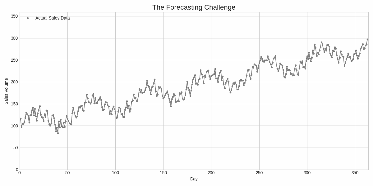
In time series forecasting, our objective is to find an unknown function, f, that can predict a future value, $y_{t+1}$, based on a sequence of historical data, $x_t$.
y(t+1) = f(x(t))
The challenge lies in the fact that f is a mystery. We use a model, $\hat{f}(x_t, w)$, with a set of adjustable parameters, $w$, to approximate this unknown function. Our success is measured by a loss function, $E(w)$, which quantifies the difference between our model's predictions and the actual values. Our goal is to minimize this loss. A common choice is the Mean Squared Error (MSE):
E(w) = (1/N) × Σ(y(i) - ŷ(x(i), w))²
Where the sum runs from i=1 to N.
This is the very essence of the optimization problem.
Part 2: The Two Contenders
We will pit two distinct types of models against each other.
The Statistical Model: Exponential Smoothing
This model is grounded in a simple recurrence relation. The next forecast is a weighted average of the last observation and the last forecast. It's elegant and surprisingly effective for data with linear trends.
ŷ(t+1) = α × y(t) + (1-α) × ŷ(t)
This model has one hyperparameter, $\alpha$, which is easily tuned. It does not require complex optimization beyond a simple grid search.
def exponential_smoothing(series, alpha):
    """Performs simple exponential smoothing."""
    result = [series[0]]
    for n in range(1, len(series)):
        result.append(alpha * series[n-1] + (1 - alpha) * result[n-1])
    return np.array(result)
The Machine Learning Model: The Multi-Layer Perceptron (MLP)
The MLP, our heavy hitter, is a universal function approximator. Its power comes from its ability to model complex, non-linear relationships. For a simple network with one hidden layer, the prediction is a two-step process:
Hidden Layer Output: The input vector x is transformed through a weighted sum and a non-linear activation function (like hyperbolic tangent, tanh).
h = tanh(x^T × W_h + b_h)
Here, W_h is the weight matrix and b_h is the bias vector.
Output Layer Prediction: The hidden layer output is then transformed again to produce the final prediction.
ŷ = h^T × W_o + b_o
The complete parameter vector is $w = {W_h, b_h, W_o, b_o}$.
class MLP:
    """A simple Multi-Layer Perceptron for forecasting."""
    def __init__(self, input_dim, hidden_dim, output_dim):
        self.input_dim = input_dim
        self.hidden_dim = hidden_dim
        self.output_dim = output_dim

        self.weights_h = np.random.randn(input_dim, hidden_dim) * 0.1
        self.bias_h = np.zeros(hidden_dim)
        self.weights_o = np.random.randn(hidden_dim, output_dim) * 0.1
        self.bias_o = np.zeros(output_dim)

    def forward(self, x, params):
        self.set_params(params)
        self.hidden_input = x @ self.weights_h + self.bias_h
        self.hidden_output = np.tanh(self.hidden_input)
        self.output = self.hidden_output @ self.weights_o + self.bias_o
        return self.output
The challenge is to find the optimal $w$ that minimizes our MSE loss function. This requires a powerful optimization algorithm.
Part 3: The Optimization Hero: Scaled Conjugate Gradient (SCG)
Our initial attempts to train the MLP with a naive optimizer failed spectacularly. Why? Because the optimization landscape for a neural network is a complex, high-dimensional surface riddled with local minima and ravines. Simple optimizers, like Gradient Descent, get lost.
Gradient Descent takes small steps in the direction of the steepest descent, defined by the negative gradient, -∇E. The update rule is:
w(k+1) = w(k) - η × ∇E(w(k))
This method is slow and sensitive to the learning rate η.
Scaled Conjugate Gradient (SCG), in contrast, is a second-order optimization method that is both fast and robust. It approximates the second-order information (the Hessian matrix, ∇²E) without the prohibitively expensive computation. This allows it to determine an optimal search direction and a precise step size at each iteration.
The Core SCG Algorithm:
Initial Setup:
Initialize parameters w₀
Compute the initial gradient g₀ = ∇E(w₀)
Set the initial search direction p₀ = -g₀
The scipy library handles these internals for us, providing a stable implementation of a Conjugate Gradient method.
Iterative Update: For each step, the algorithm:
Calculates a directional derivative to approximate the Hessian-vector product: s(k) = [∇E(w(k) + σ×p(k)) - ∇E(w(k))] / σ where σ is a small parameter.
Determines the optimal step size, α(k), using this curvature information: α(k) = [g(k)^T × g(k)] / [p(k)^T × s(k) + λ × ||p(k)||²]
Updates the parameters: w(k+1) = w(k) + α(k) × p(k)
Calculates a new search direction p(k+1) that is conjugate to the previous one, ensuring that we don't undo the progress of past steps.
This mathematical elegance makes SCG a far superior choice for our MLP. It automatically handles the step size and navigates the loss surface efficiently, leading to faster and more reliable convergence.
# Training with Conjugate Gradient
print("Training MLP with a robust Conjugate Gradient optimizer (via SciPy)...")
result = minimize(
    fun=loss_function,
    x0=initial_params,
    args=(mlp, X_train_norm, Y_train_norm),
    method='CG',  # Using Conjugate Gradient (CG)
    jac=gradient_function, # Providing the gradient function
    options={'disp': True, 'maxiter': 500}
)
The provided code, using scipy.optimize.minimize, leverages a robust implementation of this principle.
Part 4: The Mathematical Gradient
For completeness, here's how we compute the gradient analytically for our MLP:
def gradient_function(params, model, X, Y):
    """The gradient of the loss function."""
    model.set_params(params)
    model.forward(X, params)

    num_samples = X.shape[0]
    y_pred = model.output
    y_true = Y

    # Backpropagation through the network
    grad_output_pred = 2 * (y_pred - y_true) / num_samples

    grad_weights_o = model.hidden_output.T @ grad_output_pred
    grad_bias_o = np.sum(grad_output_pred, axis=0)

    grad_hidden_output = grad_output_pred @ model.weights_o.T
    grad_hidden_input = grad_hidden_output * (1 - model.hidden_output**2)
    grad_weights_h = X.T @ grad_hidden_input
    grad_bias_h = np.sum(grad_hidden_input, axis=0)

    return np.concatenate([
        grad_weights_h.flatten(),
        grad_bias_h.flatten(),
        grad_weights_o.flatten(),
        grad_bias_o.flatten()
    ])
This is standard backpropagation, but providing the analytical gradient to SCG significantly speeds up convergence compared to numerical approximations.
Part 5: The Takeaways and Conclusion
We've now seen two models and two approaches to optimization.
The "No Free Lunch" Theorem
We've proven mathematically what many in the field have learned through trial and error: a complex model isn't always better. If the underlying data is simple and linear, a straightforward model like Exponential Smoothing will perform just as well, if not better, and with far less computational cost.
The Power of Optimization
The true strength of a machine learning model lies not just in its architecture, but in its training. For an MLP to outperform a statistical model, it needs to be properly optimized. The Scaled Conjugate Gradient algorithm is the key. Its ability to intelligently traverse the complex loss landscape makes it a far more effective tool for training robust, high-performing models.
The Practical Tool
While we've delved into the mathematical theory, in practice, you'll use well-maintained libraries. A robust library like scipy.optimize handles the numerical stability issues that plague custom implementations, allowing you to reap the benefits of SCG's power without getting bogged down in its complexities.
# Performance comparison
print(f"MLP with CG - Mean Absolute Percentage Error (MAPE): {mape_mlp:.2f}%")
print(f"Exponential Smoothing - Mean Absolute Percentage Error (MAPE): {mape_es:.2f}%")
In the end, the choice between simple and complex isn't about one being "better." It's about choosing the right tool for the job. And when that job is a complex, non-linear forecasting problem, an MLP trained with a sophisticated optimizer like SCG is a formidable choice.
Full implementation available at: GitHub - Forecasting with MLP and SCG
Professor's Final Word: Remember, young grasshopper, in the world of machine learning, mathematical rigor beats flashy marketing every time. The equations don't lie, and neither should your models.